Quantize a 122B Model, One Layer at a Time
MACaQ quantizes a 122B model in 64 minutes on 32.5 GB GPU memory, one layer at a time, rest in host RAM. At 32B the inference cost is 2.3%. MACaQ-R cut KL 15% on a 35B GGUF, given the FP16 original.
Sources. The paper (arXiv 2611.10649, v1 Nov 7 2026, v2 Nov 11 2026; Huawei Cloud & AI Lab) supplies the 122B run, the Llama-3-8B ladder in its appendix and the limitations. The repository README (Apache 2.0) supplies the vLLM numbers, the MACaQ-R comparison and the command. We did not rerun anything; where a claim is ours, it says so.
The model does not fit
A 122B model, quantized in 64 minutes, peaking at 32.5 GB of GPU memory, on a single-GPU machine. That matters even if you never touch a 122B model: the same layout is what lets MACaQ-R improve a GGUF you already downloaded.
Before this, you first needed a machine that could hold 244 GB.
Qwen3.5-122B-A10B weighs 244 GB in FP16. That is 2.5× a 96 GB card. Two cards hold 192 GB, so it does not fit. Three hold 288 GB, with 44 GB to spare.
Quantization sounds like making a model smaller. But quantization is an operation that needs the model first. Rotations, calibration, Hessians: each one costs memory. Hessians here mean "how far does the output move if this weight nudges."
So the wall for large-model quantization is rarely arithmetic throughput. It is the simple fact that you have to hold the thing.
MACaQ reverses the order. Only one layer has to be on the GPU at a time. Everything else waits in host memory.
Four things below: why the old layout hits the memory wall, what the rotation costs once it moves, how the flips buy quality back, and how to improve the GGUF you already have.
Quantizing 122B means holding 122B
Start with why quantization needs a rotation at all.
Every weight matrix and activation has a few large values. Squeezing to 4 bits, one outlier stretches the shared block scale. Everything else collapses onto the same grid point.
(The 4 bits here are MXFP4: a 4-bit float where 32 values share one power-of-two scale.)
The fix is to rotate the data first. A rotation does not change what the matrix product means, but it spreads the outliers out. Every coordinate looks closer to a bell curve, and the grid starts to cover it.
The question is when the rotation happens.
QuaRot, SpinQuant and DuQuant++ are one family. They fuse the rotation into the neighbouring layer's weights. At inference there is almost nothing extra to do, because the rotation is now part of the weight. That is the elegant part.
The bill arrives at quantization time. The rotation travels across layers, so you need to know how the model is wired: where the attention output projection sits, where the residual comes back in. Different architecture, different fusion.
And once layers depend on each other, you cannot quantize one at a time.
Whether you pay at quantization time or at inference is the real fork in this field.
Table 1: where each method keeps the rotation
| Method | Rotation lives | Cross-layer at quant time | One layer at a time | Inference cost |
|---|---|---|---|---|
| QuaRot | fused into the next layer's weights | yes | no | almost nothing extra |
| SpinQuant | fused, with learned rotations | yes | no | almost nothing extra |
| DuQuant++ | fused into the next layer's weights | yes | no | almost nothing extra |
| MACaQ | online, at inference | no | yes | +2.3% |
Table 1 is a conceptual map, not the paper's benchmark list. This essay compares against DuQuant++ and MR-GPTQ only; the paper also benchmarks QuaRot and FlatQuant.
The map says one thing: the rotation itself is not smarter, it just runs at a different time. The quality comes later, from the flips.
Moving the rotation to inference time
MACaQ takes the other branch. The rotation stays out of the weights and runs at inference.
Each layer's incoming activations get a per-channel scale, then a block-Hadamard transform. Hadamard is a fast, invertible linear map whose job is to flatten outliers.
The inverse is absorbed into the weights at quantization time. The arithmetic is equivalent. The same multiply just moves from the quantizer to the runtime.
The interesting consequence is not the saving, it is who depends on whom. With the rotation online, a layer needs only its own weights and its own activation statistics. Nothing points backwards.
So quantization can stream: load a layer onto the GPU, quantize it, write it out, free it, load the next. The paper calls this streaming with lazy loading, and puts it in one sentence; the remaining weights stay in host memory, and only the layer being processed has to sit on the GPU.
Table 2: the Qwen3.5-122B-A10B run
| Item | Value |
|---|---|
| Parameters | 122B (mixture-of-experts; about 10B active per token) |
| FP16 weights | about 244 GB |
| Machine | one 96 GB GPU (the paper lists 504 TFLOPS FP16 and 1.79 TB/s, not a model name) |
| Peak GPU memory while quantizing | 32.5 GB |
| Quantization time | 64 minutes (32 flips, 512K calibration tokens) |
| WikiText-2 perplexity | 5.14 (FP16 is 5.06) |
| Footprint of the result | 74 GB; runs on the same card |
Figure 1, left: the rotation travels with the layers, so quantizing two of them couples them. Right: the rotation stays online, so one layer is on the GPU at a time.
The number people misread is 32.5 GB. That is device memory at its peak, not the whole footprint. The 244 GB of FP16 weights is still in host memory; it is just never resident on the GPU at once.
So the real requirement is a big enough card plus a big enough host. Not "32.5 GB is enough." Almost every repost drops that half.
No architecture changes, either. The repo lists FLUX.2 Klein 4B for images, Wan2.2 for video and stable-audio for audio. The paper itself demonstrates one image model and describes the method as applying "without architecture-specific modifications."
If you keep a zoo of models, that portability matters more than the 64 minutes.
The bill: 2.3%
The online transform is not free. Against pure MXFP4, MACaQ adds 2.3% end-to-end on Qwen3-32B in vLLM. The paper never measures the 122B run; that is a 32B number.
The paper's Figure 3 breaks it down: the cost is measured on decode, batch 1, context 512. It shrinks as models grow, because bigger matrices take longer and a few extra multiplies weigh less.
I think what that 2.3% buys is "you do not have to understand the architecture." That is the hinge of the design.
The other number that gets mangled is in Table 3: W4A4 (4-bit weights, 4-bit activations) on Qwen3.8-27B in vLLM, a serving engine. MACaQ runs at 2.33× prefill and 2.58× decode.
Those are throughput ratios against BF16, not against pure MXFP4. The two denominators answer different questions; mixing them wrecks the paragraph.
Table 3: Qwen3.8-27B in vLLM (README; BF16 = 1.00×)
| Precision | Perplexity ↓ (README; dataset unstated) | prefill | decode |
|---|---|---|---|
| BF16 | 2.8463 | 1.00× | 1.00× |
| MACaQ W4A4 | 2.8994 | 2.33× | 2.58× |
Perplexity goes from 2.8463 to 2.8994, a 1.9% increase. That is not lossless; it is lossy and cheap, which is a different claim.
Table 3 comes from the README and is a different experiment from Table 2. Do not compare across tables.
The rounding is the easy part
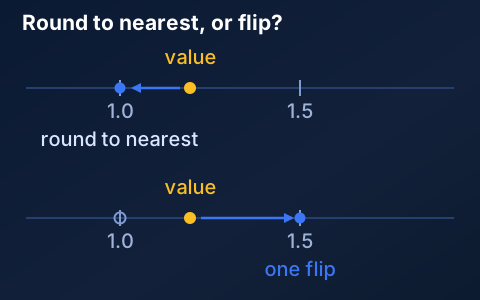
Four bits give you a small grid. Round-to-nearest (RTN) picks the closest point. It looks only at the weight itself.
MACaQ does one more thing: it flips a code.
A flip moves a single FP4 code to an adjacent representable value. Not a re-quantization, just a different point in the same grid.
Whether to flip is decided by the whole layer's loss. A Hessian approximation asks how far the output moves if this code changes. Then it flips greedily, one code at a time.
Why is that cheap? The only candidates are the neighbour on the left and the neighbour on the right. The search space is tiny. No continuous optimization.
Two knobs control it: how many flips, and how many calibration tokens. Fast means few flips, good means many. Table 4 is the appendix ladder on Llama-3-8B.
Table 4: the trade on Llama-3-8B (MXFP4 W4A4, WikiText-2 perplexity)
| Setting | Time | Perplexity ↓ |
|---|---|---|
| FP16 (reference) | — | 6.14 |
| RTN only | 2.2 s | 8.29 |
| MACaQ, 0 flips (rotation + exponent screen) | 5.5 s | 7.64 |
| MACaQ, 1 calibration block (2048 tokens) | 14.8 s | 7.11 |
| MACaQ, 128 flips, 31 blocks | 88.1 s | 6.91 |
| MACaQ, 512 flips, 977 blocks | 636.9 s | 6.85 |
| MR-GPTQ, 128 blocks | 319.1 s | 7.11 |
| DuQuant++ (GPTQ), 128 blocks | 624.4 s | 7.16 |
The MACaQ rows are points on one curve with different calibration budgets. The MR-GPTQ and DuQuant++ rows use 128 blocks each. Do not read down the time column and call it a race; those are different budgets. The paper's own fair comparison is 128 flips and about 200K tokens, roughly 150 s on Llama-3-8B, landing at 6.90.
This table is more useful than a headline ratio: you can pick your own row.
The abstract claims MACaQ "already matches their best perplexity on Llama-3-8B in 11× less quantization time." We did not collapse that into a single ratio: Table 4 is a set of single points, the abstract is describing a curve. For a decision, read the table.
Figure 2: rounding picks the nearest point. A flip moves one code to the neighbour, and the layer's loss decides whether that happens.
One thing to say plainly: this is not lossless 4-bit. Even the best setting goes from 6.14 to 6.85, about 12% worse perplexity. RTN is 8.29. Both are lossy. The difference is how much, and whether you will pay the time.
Fixing the GGUF you already have
Everything above is "quantize a model from scratch." Most people are not doing that. They have a folder of downloaded GGUFs.
MACaQ-R is for that case. Take an existing GGUF and its original FP16 file as a teacher, run one refine pass.
The weight codes get rewritten. The native format and block scales stay. So the result still runs on a stock llama.cpp build.
Table 5: Qwen3.6-35B-A3B before and after MACaQ-R (README, single run)
| Version | GGUF size | KL to FP16 ↓ |
|---|---|---|
| Unsloth UD-Q4_K_XL | 22.36 GB | 0.015731 |
| MACaQ-R Q4_K_XL | 22.36 GB | 0.013367 |
KL divergence measures how far two distributions are apart; lower is better. Same size, 0.015731 down to 0.013367, a 15.0% drop. Same file size, same runtime, different code in each slot.
The command is straight from the README:
.venv-llamacpp/bin/python llamacpp/macaq.py refine \
  --model models/model-q4.gguf --hf models/original \
  --teacher models/original-f16.gguf --calibration data/calibration.txt \
  --output models/model-macaq-r.gguf --work-dir work/refinement
Then it runs, with nothing to swap in the backend:
llama cli -m models/model-macaq-r.gguf
llama.cpp binaries changed names across versions. Older builds use llama-cli; use whichever you installed.
Simple command, not-simple prerequisites. Three of them, from the README:
- Python 3.12, and a separate environment per backend. Not just
pip install - The original FP16 file as teacher. If all you have is the GGUF, you stop here
- A calibration text file and the original weights directory
One more limit. Table 5 is a single comparison: one model, one baseline. Do not generalize it to "any GGUF improves by 15%." Yours may improve more, or not at all. Measure KL yourself.
How fast it runs afterwards is a separate topic, decided by bit width and kernel. We covered that in Quantization Speed Is Often a Kernel Problem.
What this does not prove
The paper puts the cost in the first line of Limitations. A layer-local design means cross-layer error compensation is impossible. A second pass over cross-layer statistics would likely bring back the slow quantization of the other methods. That is a design trade, not an oversight.
Also worth knowing:
- No third-party replication yet. First posted Nov 7; the DuQuant++ and MR-GPTQ comparisons were run by the authors
- W4A4 numbers are concentrated on a few models. Do not read the +1.9% on Qwen3.8-27B as a general result
- MoE: expert layers only. Embeddings and lm-head are skipped in every model, not just MoE
- The 122B budget differs from the rest. 32 flips and 512K calibration tokens; the fair comparison used 128 flips and about 200K tokens
- Qwen3.5 / 3.6 / 3.8 are different generations. Do not cross-compare
- Ascend is not plug and play. Needs CANN and
torch_npu; upstream has kernel PRs only, and full-model execution still needs a serving runtime - 32.5 GB is device memory, not the whole footprint. Your host still has to hold 244 GB
And the +2.3% again: it is measured against pure MXFP4. Against BF16 the same method is over 2× faster (Table 3). Same method, different denominator, opposite headline.
Three things to do tomorrow
- Measure a baseline first. If you own a GGUF, compute KL against its FP16 original. The README does not give you a KL script; you will have to find one. Without a baseline, "15% lower" is somebody else's number. Check the file is not broken first, too: Your quantized model might be broken.
- Run one refine pass. If you have the original, run it, then run the same prompt on your usual llama.cpp build and compare outputs. Worst case you lose one refine.
- Quantizing something 100B-class is a single-GPU job now. Provided the host can hold the FP16 weights.
The gate moved. It used to be a card. Now it is a machine.